Building Blocks of Deep Learning
Complex neural networks
One layer
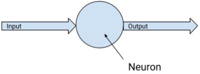
- Each neuron: Output = (Weight * Input) + Bias
```python linenums=”1” my_layer = keras.layers.Dense(units=1, input_shape=[1]) model = tf.keras.Sequential([my_layer]) model.compile(optimizer=’sgd’, loss=’mean_squared_error’)
xs = np.array([-1.0, 0.0, 1.0, 2.0, 3.0, 4.0], dtype=float) ys = np.array([-3.0, -1.0, 1.0, 3.0, 5.0, 7.0], dtype=float)
model.fit(xs, ys, epochs=500) ```
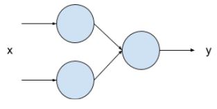
Two layers
- Two layers
- First layer with two neurons
- Second layer with one neurons
Code setup
```python linenums=”1” my_layer_1 = keras.layers.Dense(units=2, input_shape=[1]) my_layer_2 = keras.layers.Dense(units=1)
model = tf.keras.Sequential([my_layer_1, my_layer_2]) model.compile(optimizer=’sgd’, loss=’mean_squared_error’)
xs = np.array([-1.0, 0.0, 1.0, 2.0, 3.0, 4.0], dtype=float) ys = np.array([-3.0, -1.0, 1.0, 3.0, 5.0, 7.0], dtype=float)
model.fit(xs, ys, epochs=500) ```
- Each neuron in the first layers has its own weight/bias and will general one output.
- The sole neuron in the second layers will have two inputs, which means it will have two weight and one bias.
Manual output calculation
```python linenums=”1” value_to_predict = 10.0
layer1_w1 = (my_layer_1.get_weights()[0][0][0]) layer1_w2 = (my_layer_1.get_weights()[0][0][1]) layer1_b1 = (my_layer_1.get_weights()[1][0]) layer1_b2 = (my_layer_1.get_weights()[1][1])
neuron1_output = (layer1_w1 * value_to_predict) + layer1_b1 neuron2_output = (layer1_w2 * value_to_predict) + layer1_b2
layer2_w1 = (my_layer_2.get_weights()[0][0]) layer2_w2 = (my_layer_2.get_weights()[0][1]) layer2_b = (my_layer_2.get_weights()[1][0])
neuron3_output = (layer2_w1 * neuron1_output) + (layer2_w2 * neuron2_output) + layer2_b print(neuron3_output) ```
Question: Validating manual output
- Implement the two-layer code setup and the manual output calculation.
- Match the manual result with the
model.predictcall for comparison purposes.
Question: Comparing models
- Comparing the results of one-layer and two-layer setup.
- Which one is better?
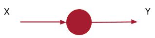
Introduction to classification
Overview
- Previously: Regression
- Fit internal parameters of a function, from X to Y
- Using neural network to predict a single value from one or more inputs.
- Another scenario: Classification
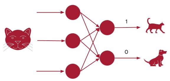
- Output:
- Dog: [0,1]
- Cat: [1,0]
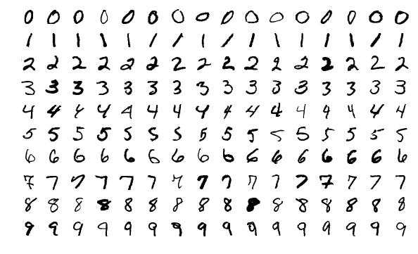
Example: Hand writing recognition
- Output definitions:
- [
1,0,0,0,0,0,0,0,0,0,0]: represent images similar to number 0 - [0,
1,0,0,0,0,0,0,0,0,0]: represent images similar to number 1 - [0,0,
1,0,0,0,0,0,0,0,0]: represent images similar to number 2 - [0,0,0,0,
1,0,0,0,0,0,0]: represent images similar to number 3 - [0,0,0,0,0,
1,0,0,0,0,0]: represent images similar to number 4 - [0,0,0,0,0,0,
1,0,0,0,0]: represent images similar to number 5 - [0,0,0,0,0,0,0,
1,0,0,0]: represent images similar to number 6 - [0,0,0,0,0,0,0,0,
1,0,0]: represent images similar to number 7 - [0,0,0,0,0,0,0,0,0,
1,0]: represent images similar to number 8 - [0,0,0,0,0,0,0,0,0,0,
1]: represent images similar to number 9
- [
Dataset
- MNIST dataset, built into Tensorflow
- Already split into training and validation images and labels
- 60,000 labelled training examples
- 10,000 labelled validation examples
- Each image in MNIST
- 28 by 28 pixels
- Each pixel is monochrome, therefore the value is 0 to 255
- Load data:
```python linenums=”1” import sys import tensorflow as tf
data = tf.keras.datasets.mnist (training_images, training_labels), (val_images, val_labels) = data.load_data()
training_images = training_images / 255.0 val_images = val_images / 255.0 ```
- Lines 5 and 6: normalize pixel values to between 0 and 1.
Build the model
```python linenums=”1” model = tf.keras.models.Sequential([tf.keras.layers.Flatten(input_shape=(28,28)), tf.keras.layers.Dense(20, activation=tf.nn.relu), tf.keras.layers.Dense(10, activation=tf.nn.softmax)]) model.compile(optimizer=’adam’, loss=’sparse_categorical_crossentropy’, metrics=[‘accuracy’]) model.fit(training_images, training_labels, epochs=20, validation_data=(val_images, val_labels))
1
2
3
4
5
6
7
8
9
10
11
12
13
14
15
16
17
18
19
20
21
22
23
24
25
26
27
28
29
30
31
32
33
34
35
36
37
38
39
40
41
42
43
44
45
46
47
48
49
50
51
52
53
54
55
56
57
58
59
60
61
62
63
64
65
66
67
68
69
70
71
72
73
74
75
76
77
78
79
80
81
82
83
84
85
86
87
88
89
90
91
92
93
94
95
96
97
98
99
100
101
102
103
104
105
106
107
108
109
110
111
112

- Line 1: Flatten the 28x28 image into something that fit into the the Dense layers


<figure

>
  <picture>
    <!-- Auto scaling with imagemagick -->
    <!--
      See https://www.debugbear.com/blog/responsive-images#w-descriptors-and-the-sizes-attribute and
      https://developer.mozilla.org/en-US/docs/Learn/HTML/Multimedia_and_embedding/Responsive_images for info on defining 'sizes' for responsive images
    -->

    <img
      src="/assets/img/courses/csc574/03-dl/flatten_01.webp"


        width="50%"


        height="auto"


        data-zoomable


        loading="lazy"

      onerror="this.onerror=null; $('.responsive-img-srcset').remove();"
    >
  </picture>


</figure>


- This is so that each image data can be fed into the next Dense layer (fully connected)


<figure

>
  <picture>
    <!-- Auto scaling with imagemagick -->
    <!--
      See https://www.debugbear.com/blog/responsive-images#w-descriptors-and-the-sizes-attribute and
      https://developer.mozilla.org/en-US/docs/Learn/HTML/Multimedia_and_embedding/Responsive_images for info on defining 'sizes' for responsive images
    -->

    <img
      src="/assets/img/courses/csc574/03-dl/flatten_02.webp"


        width="50%"


        height="auto"


        data-zoomable


        loading="lazy"

      onerror="this.onerror=null; $('.responsive-img-srcset').remove();"
    >
  </picture>


</figure>


- Line 2: Our first Dense layer which has 20 neurons
    - How to pick optimum number
        - Too few: not enough to learn about the image
        - Too many: over specialize, slow to learn
- Line 3: Our final Dense layer with 10 neurons
    - Expected 10 values for the output list.
- Lines 2 and 3: Activation function
    - Called by each neuron
    - The `ReLU` activation function changes any output that is less than 0 to 0.
        - Commonly used in dense layers,
        - Introduce a non-linear relationship between the layers to help capturing complex relationships
    - The `softmax` activation function helps finding the neuron from amongst the 10 that
    has the highest value.
- Lines 4, 5, 6: Compiling
    - `Adam` optimizer can vary its learning rate to help with faster convergence.
    - The selected loss function measure loss for categorical data.
- Line 7: Training
    - 20 epochs
    - train on `training_images` and `training_labels`
    - `val_images` and `val_labels` are kept for validation

```python linenums="1"
model.evaluate(val_images, val_labels)

classifications = model.predict(val_images)
print(classifications[0])
print(val_labels[0])