Machine Learning Paradigm

Overview and motivation

Example

• A new paradigm for programming
  • Explicitly coding a solution vs Implicitly learning a solution

Example: Explicit coding: pong

• It is how we do it since the beginning of time!

• The ball moves along a path
  • Angle/velocity
• The ball hits
  • A paddle or a wall
  • Change of angle/velocity
• We can code these behaviors based on physical rules + game rules
  • Rules are predetermined by the programmer, then coded and tested. Everything needs to be figured out in advance.
  • Complexity scale with code amount

Explicit coding

• Powerful but can be limited

Explicit coding example: activity detection

• Write an app that uses sensors on a phone or a watch or something else to determine a person’s activity.
  • Use the data about their speed and write a rule that determines if the speed is below a certain amount, then they’re probably walking.

Walking

• If less than 4 miles an hour, then they are walking.

1
2
 
if speed < 4.0:
    print("Walking")
 

Running

• If more than 4 miles an hour, then they are running.

1
2
3
4
 
if speed < 4.0:
    print("Walking")
else:
    print("Running")
 

Biking

• If more than 4 miles an hour but less than 12, then they are running.
• Otherwise, they are biking

1
2
3
4
5
6
 
if speed < 4.0:
    print("Walking")
elif speed < 12.0:
    print("Running")
else
    print("Biking")
 

failure Playing soccer

• How do we describe movements of soccer players? goal keeper?

• It is challenging to write rules for complex problems

Implicit learning

Machine Learning Paradigm

• In a nutshell:
  • Make a guess about the relationship between the data and its labels
    • low speed + long distance or short distance + along road + few stops = walking
    • low speed + long distance + on a field + regular stops = golfing
    • low or high speed + long distance + enclosed area = soccer
  • Measures how good or how bad that guess is.
    • Terminology: loss
    • Higher loss implies lower accuracy.
    • Measure the results of your guess,
    • Use the data from the accuracy measurement to estimate next guess, optimizing based on what you already know.
  • Repeat the process
    • Assumption: each subsequent guess gets better than the previous one

Example: Relationship between two sets of numbers

• X: $-1,0,1,2,3,4$
• Y: $-3,-1,1,3,5,7$

First guess

• $x_1=-1$ and $y_1=-3$
  • $y_1 = 3{x}_1$
• $Y = 3X$
  • Guess: $-3,0,3,6,9,12$
  • Expected: Y: $-3,-1,1,3,5,7$

Second guess

• $x_1=-1$ and $y_1=-3$
  • $y_1 = 3x_1$
• $x_2=0$ and $y_1=-1$
  • $y_2 = x_2 - 1$
• $Y = 3X - 1$
  • Guess: $-4,-1,2,5,8,11$
  • Expected: Y: $-3,-1,1,3,5,7$

Third guess

• $x_1=-1$ and $y_1=-3$
  • $y_1 = 3x_1$
• $x_2=0$ and $y_1=-1$
  • $y_2 = x_2 - 1$
• $x_3=1$ and $y_3=2$
  • $y_3 = 2x_3$
• $Y = 2X - 1$
  • Guess: $-3,-1,1,3,5,7$
  • Expected: Y: $-3,-1,1,3,5,7$

Measure accuracy

Setting up programming environment

• Open the ml-paradigm.ipynb notebook from the tinyml Git repo (python/notebooks).
  • Select tinyml as the kernel for the notebook.

Example: Coding hands on

• Run the following code segment in a cell and monitor different combinations of w and b to observe the loss value

1
2
3
4
5
6
7
8
9
10
11
12
13
14
15
16
17
18
19
20
21
22
23
24
25
26
27
28
29
30
31
32
33
34
35
36
37
38
39
 
import math
import matplotlib.pyplot as plt
import numpy as np

w = 3
b = -1

x = [-1, 0, 1, 2, 3, 4]
y = [-3, -1, 1, 3, 5, 7]
myY = []

for thisX in x:
  thisY = (w*thisX)+b
  myY.append(thisY)

print(f"Real Y is {str(y)}")
print(f"My Y is   {str(myY)}")

# Sample data
x = np.array(x)
y = np.array(y)
myY = np.array(myY)

plt.plot(x, y, 'o')  # Plot points as circles
plt.plot(x, myY, 'o')  # Plot points as circles

# Add vertical lines
for i in range(len(x)):
    plt.vlines(x[i], y[i], myY[i], linestyles='dashed')
    length = y[i] - myY[i]
    plt.text(x[i], (y[i] + myY[i]) / 2, f"{length:.2f}", ha='center', va='center')

# Add gridlines
plt.grid(True)

plt.xlabel('X-axis')
plt.ylabel('Y-axis')
plt.title('Points with Vertical Lines')
plt.show()
 

How good (or bad) are your guesses?

• We want to have a way to measure the loss values and their aggregation.
• Account for negative value (over/under guess)
• Run the following code in the next cell of your notebook

1
2
3
4
5
6
7
8
9
10
11
12
13
14
15
16
17
18
19
20
21
22
23
24
25
 
import math

w = 3
b = -1

x = [-1, 0, 1, 2, 3, 4]
y = [-3, -1, 1, 3, 5, 7]
myY = []


for thisX in x:
  thisY = (w*thisX)+b
  myY.append(thisY)

print(f"Real Y is {str(y)}")
print(f"My Y is   {str(myY)}")

# let's calculate the loss
total_square_error = 0
for i in range(0, len(y)):
  square_error = (y[i] - myY[i]) ** 2
  total_square_error += square_error

print(f"My loss is: {str(math.sqrt(total_square_error))}")

 

Loss function

Loss function: Mean Squared Error (MSE)

$J = \frac{1}{n}\sum(actual-predicted)^2$

• Given the following
  • Set of X: $x_0,x_1,…,x_n$
  • Set of Y (actual): $y_0,y_1,…y_n$
  • A linear regression function that try to estimate Y from X: $Y=mX + c$

MSE loss function for linear regression

$J = \frac{1}{n}\sum^{n}_{i=0} (y_i - (mx_i+c))^2$

Run the below code in another cell of the notebook and examine how the MSE loss function changes as we change the parameters of our estimation function.

1
2
3
4
5
6
7
8
9
10
11
12
13
14
15
16
17
18
19
20
21
22
23
24
25
26
27
28
29
30
31
32
33
 
import numpy as np
import matplotlib.pyplot as plt
from mpl_toolkits.mplot3d import Axes3D

# Generate some sample data
np.random.seed(0)
X = 2 * np.random.rand(100, 1)
y = 4 + 3 * X + np.random.randn(100, 1)

# Define a function to compute the loss
def compute_loss(w0, w1):
    y_pred = w0 + w1 * X
    return np.mean((y - y_pred) ** 2)

# Create a grid of parameter values
w0_range = np.linspace(-10, 10, 50)
w1_range = np.linspace(-10, 10, 50)
W0, W1 = np.meshgrid(w0_range, w1_range)

# Compute the loss for each combination of parameter values
loss = np.zeros_like(W0)
for i in range(len(w0_range)):
    for j in range(len(w1_range)):
        loss[i, j] = compute_loss(W0[i, j], W1[i, j])

# Plot the 3D surface
fig = plt.figure()
ax = fig.add_subplot(111, projection='3d')
ax.plot_surface(W0, W1, loss, cmap='viridis')
ax.set_xlabel('w0 (intercept)')
ax.set_ylabel('w1 (slope)')
ax.set_zlabel('Loss')
plt.show()
 

Gradient

• Gradient: measure of change in all the weights (m and c in the case of linear regression) with regard to change in error.
  • Slope of the loss function: Calculated as the derivative of the loss function with respect to the specific weight being calculated.
• $D_m = \frac{\partial J}{\partial m} = \frac{1}{n} \sum_{i=1}^{n} 2(y_i - (mx_i + c)) \cdot \frac{\partial}{\partial m}(y_i - (mx_i + c)) = \frac{1}{n}\sum^{n}_{i=0} 2(y_i - (mx_i+c))(-x_i)$
• $D_c = \frac{\partial J}{\partial c} = \frac{-2}{n}\sum^{n}_{i=0} (y_i - (mx_i+c))$

Gradient descent

• Gradient descent:
  • Iterative function that applies a predefined rate of change (learning rate $L$) to m and c until a perceived minimal loss is realized.
• L = learning rate < 1
• $m = m - LD_m$
• $c = c - LD_c$

Gradient descent in TensorFlow

Implementing gradient descent calculation from scratch is a tedious process. It involves:

• Identifying and implementing the mathematical derivation (calculus) of your original function.
• Setting up loops to support repeated calculations of gradients as you iteratively optimize your model parameters.

The TensorFlow library includes various utility APIs that support automated mathematical subsystems to help streamlining this process.

• GradientTape is one such API that support automatic differentiation.

More details about GradientTape are included in the the ml-paradigm_minimizing_loss.ipynb notebook. - Select the tinyml kernel when open this notebook.

Introductory neural network

Up to this point, we have been manually guessing values for $m$ and $c$ because we knew our data was generated by a simple linear function ($Y=mX+c$)

But what if we don’t know the mathematical function that describes the data?

In real-world scenarios like detecting a pothole or recognizing a voice, the underlying math is often too complex to define with a single equation.

This is where we use a Neural Network. Instead of trying to find the parameters of a specific, known function, we allow the network to estimate its own internal parameters (weights).

Through a repeated cycle of Guessing, Measuring, and Optimizing, the network learns to approximate the correct output without us ever needing to know the mathematical format of the original, unknown function.

This is also the basic concept for implicit learning.

Example: A neural network

• Hidden Layer 1: units=4
• Hidden Layer 2: units=4
• Output Layer: units=1

Let’s copy the following code into an empty cell in the ml-paradigm notebook.

• Open a new cell and run the following:
  • Press Shift-L to turn on line number in cells.

1
2
3
4
5
6
7
8
9
10
11
12
13
 
import numpy as np
import tensorflow as tf
model = tf.keras.Sequential([tf.keras.layers.Dense(units=1, input_shape=[1])])

model.compile(optimizer='sgd', loss='mean_squared_error')

xs = np.array([-1.0,  0.0, 1.0, 2.0, 3.0, 4.0], dtype=float)
ys = np.array([-3.0, -1.0, 1.0, 3.0, 5.0, 7.0], dtype=float)

model.fit(xs, ys, epochs=500)

print(model.predict(np.array([10.0])))
print(model.predict(np.array([10.0, 11.0])))
 

• Line 3 defines a very simple neural network model.
  • units= 1: Dimensionality of the output space
  • input_shape=[1]: Dimensionality of the input data
    • We’re training a neural network on single x’s to predict single y’s.
• Line 5 compiles the model
  • Optimizer is defined as sgd - Stochastic Gradient Descent.
  • Loss function is mean_squared_error - MSE.
• Lines 7 and 8 define the X and Y arrays to train the models.
• The fitting process runs 500 times (500 epochs)
  • Each epoch is a step:
    • Guess
    • Measure the loss
    • Optimize and repeat
• We can observe the predicted output by feeding a single value (line 12) or an array of values (line 13)

Common Layer Type

• Dense Layer: neurons from previous layer fully connected to neurons in the next layer
• Convolutional Layer: contain filters that can be used to transform data
• Recurrent Layer: allow learning about relationship between data points in a sequence.

Exercise

• Replace SHAPE and LOSS with relevance values for the following segment of code, then run it in a new cell

1
2
3
4
5
6
7
8
9
10
11
12
13
14
15
16
17
18
19
20
21
22
23
24
25
26
27
28
29
30
 
import sys

import numpy as np
import tensorflow as tf
import matplotlib.pyplot as plt
from tensorflow.keras import Sequential
from tensorflow.keras.layers import Dense

predictions = []
class myCallback(tf.keras.callbacks.Callback):
def on_epoch_end(self, epoch, logs={}):
    predictions.append(model.predict(xs))
callbacks = myCallback()

# We then define the xs (inputs) and ys (outputs)
xs = np.array([-1.0, 0.0, 1.0, 2.0, 3.0, 4.0], dtype=float)
ys = np.array([-3.0, -1.0, 1.0, 3.0, 5.0, 7.0], dtype=float)

SHAPE = #YOUR CODE HERE#
LOSS = #YOUR CODE HERE#

model = Sequential([Dense(units=1, input_shape=SHAPE)])
model.compile(optimizer='sgd', loss=LOSS)
model.fit(xs, ys, epochs=300, callbacks=[callbacks], verbose=2)
EPOCH_NUMBERS=[1,25,50,150,300] # Update me to see other Epochs
plt.plot(xs,ys,label = "Ys")
for EPOCH in EPOCH_NUMBERS:
    plt.plot(xs,predictions[EPOCH-1],label = "Epoch = " + str(EPOCH))
plt.legend()
plt.show()
 

Complex neural network

One layer

• Each neuron: Output = (Weight * Input) + Bias

1
2
3
4
5
6
7
8
 
my_layer = keras.layers.Dense(units=1, input_shape=[1])
model = tf.keras.Sequential([my_layer])
model.compile(optimizer='sgd', loss='mean_squared_error')

xs = np.array([-1.0,  0.0, 1.0, 2.0, 3.0, 4.0], dtype=float)
ys = np.array([-3.0, -1.0, 1.0, 3.0, 5.0, 7.0], dtype=float)

model.fit(xs, ys, epochs=500)
 

Two layers

• Two layers
  • First layer with two neurons
  • Second layer with one neurons

Code setup

```python linenums=”1” my_layer_1 = keras.layers.Dense(units=2, input_shape=[1]) my_layer_2 = keras.layers.Dense(units=1)

model = tf.keras.Sequential([my_layer_1, my_layer_2]) model.compile(optimizer=’sgd’, loss=’mean_squared_error’)

xs = np.array([-1.0, 0.0, 1.0, 2.0, 3.0, 4.0], dtype=float) ys = np.array([-3.0, -1.0, 1.0, 3.0, 5.0, 7.0], dtype=float)

model.fit(xs, ys, epochs=500) ```

• Each neuron in the first layers has its own weight/bias and will general one output.
• The sole neuron in the second layers will have two inputs, which means it will have two weight and one bias.

Manual output calculation

1
2
3
4
5
6
7
8
9
10
11
12
13
14
15
16
 
value_to_predict = 10.0

layer1_w1 = (my_layer_1.get_weights()[0][0][0])
layer1_w2 = (my_layer_1.get_weights()[0][0][1])
layer1_b1 = (my_layer_1.get_weights()[1][0])
layer1_b2 = (my_layer_1.get_weights()[1][1])

neuron1_output = (layer1_w1 * value_to_predict) + layer1_b1
neuron2_output = (layer1_w2 * value_to_predict) + layer1_b2

layer2_w1 = (my_layer_2.get_weights()[0][0])
layer2_w2 = (my_layer_2.get_weights()[0][1])
layer2_b = (my_layer_2.get_weights()[1][0])

neuron3_output = (layer2_w1 * neuron1_output) + (layer2_w2 * neuron2_output) + layer2_b
print(neuron3_output)
 

Question: Validating manual output

• Implement the two-layer code setup and the manual output calculation.
• Match the manual result with the model.predict call for comparison purposes.

Question: Comparing models

• Comparing the results of one-layer and two-layer setup.
• Which one is better?

Introduction to classification

Overview

• Previously: Regression
  • Fit internal parameters of a function, from X to Y
  • Using neural network to predict a single value from one or more inputs.

• Another scenario: Classification

• Output:
  • Dog: [0,1]
  • Cat: [1,0]

Example: Hand writing recognition

• Output definitions:
  • [1,0,0,0,0,0,0,0,0,0,0]: represent images similar to number 0
  • [0,1,0,0,0,0,0,0,0,0,0]: represent images similar to number 1
  • [0,0,1,0,0,0,0,0,0,0,0]: represent images similar to number 2
  • [0,0,0,0,1,0,0,0,0,0,0]: represent images similar to number 3
  • [0,0,0,0,0,1,0,0,0,0,0]: represent images similar to number 4
  • [0,0,0,0,0,0,1,0,0,0,0]: represent images similar to number 5
  • [0,0,0,0,0,0,0,1,0,0,0]: represent images similar to number 6
  • [0,0,0,0,0,0,0,0,1,0,0]: represent images similar to number 7
  • [0,0,0,0,0,0,0,0,0,1,0]: represent images similar to number 8
  • [0,0,0,0,0,0,0,0,0,0,1]: represent images similar to number 9

Dataset

• MNIST dataset, built into Tensorflow
  • Already split into training and validation images and labels
  • 60,000 labelled training examples
  • 10,000 labelled validation examples
• Each image in MNIST
  • 28 by 28 pixels
  • Each pixel is monochrome, therefore the value is 0 to 255

Build the model

1
2
3
4
5
6
7
8
9
10
11
12
13
14
15
16
17
18
19
20
21
22
23
24
 
import tensorflow as tf
import matplotlib.pyplot as plt

data = tf.keras.datasets.mnist
(training_images, training_labels), (val_images, val_labels) = data.load_data()

training_images  = training_images / 255.0
val_images = val_images / 255.0

model = tf.keras.models.Sequential([tf.keras.layers.Flatten(input_shape=(28,28)),
                                    tf.keras.layers.Dense(20, activation=tf.nn.relu),
                                    tf.keras.layers.Dense(10, activation=tf.nn.softmax)])
model.compile(optimizer='adam',
              loss='sparse_categorical_crossentropy',
              metrics=['accuracy'])
model.fit(training_images, training_labels, epochs=20, validation_data=(val_images, val_labels))
model.evaluate(val_images, val_labels)

plt.figure(figsize=(3, 3))
plt.imshow(val_images[0], cmap='gray')

classifications = model.predict(val_images)
print(classifications[0])
print(val_labels[0])
 

• Lines 4 and 5: Load MNIST dataset from Tensorflow.
  • We split our dataset into two portions, training and validation.
  • We use training data to train (adjust) the weights and biases on the neurons.
  • We use validation data to test (validate) on how actually good these weights and biases are on unseen data.
• Lines 7 and 8: normalize pixel values to between 0 and 1.
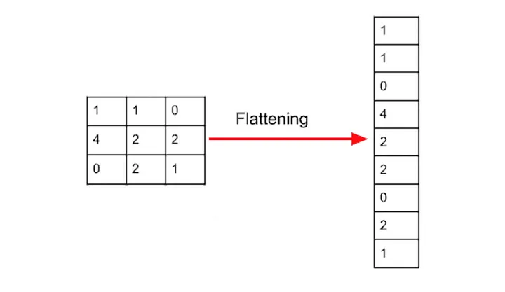
• Line 10: Adding the Flatten layer to the model to turn the 2D matrix representing the image into a one-dimensional vector.

• This so that each image data can be fed into the subsequent Dense layers.

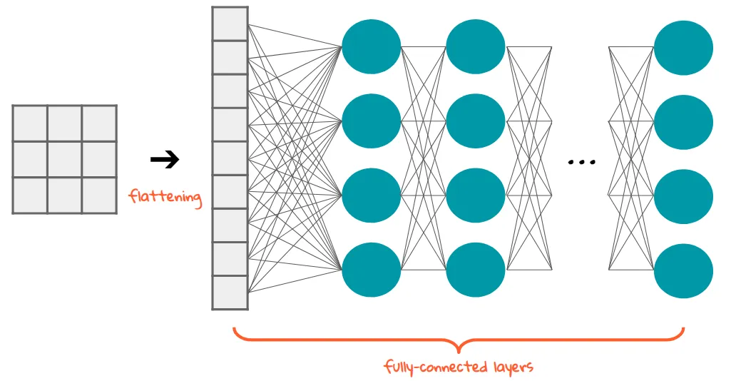
• Line 11: Our first Dense layer which has 20 neurons
  • How to pick optimum number
    • Too few: not enough to learn about the image
    • Too many: over specialize, slow to learn
• Line 12: Our final Dense layer with 10 neurons
  • Expected 10 values for the output list.
• Lines 11 and 12: Activation function
  • Called by each neuron
  • The ReLU activation function changes any output that is less than 0 to 0.
    • Commonly used in dense layers,
    • Introduce a non-linear relationship between the layers to help capturing complex relationships
  • The softmax activation function helps finding the neuron from amongst the 10 that has the highest value.
• Lines 13, 14, 15: Compiling
  • Adam optimizer can vary its learning rate to help with faster convergence.
  • The selected loss function measure loss for categorical data.
• Line 16: Training
  • 20 epochs
  • train on training_images and training_labels
  • val_images and val_labels are kept for validation
• Lines 19 and 20:
  • Visualizing the actual image that we are trying to classify.
• Lines 22, 23, and 24:
  • Printing the predicted label (classification) generated by the neural network.